Principal Component Analysis

Principal Component Analysis (PCA) is a dimensionality reduction technique used in data analysis and machine learning. It transforms a large set of variables into a smaller one that still contains most of the original information.

PCA identifies the directions (called principal components) along which the variation in the data is maximized. These components are linear combinations of the original features and are orthogonal to each other.

Typical reasons for using this are:

• To reduce the number of features while preserving as much variance as possible.
• To improve model performance and reduce overfitting.
• To visualize high-dimensional data in 2D or 3D.
• To eliminate correlated or redundant features.

Code Example (using sklearn)

import numpy as np
import matplotlib.pyplot as plt
from sklearn.decomposition import PCA
from sklearn.datasets import load_iris

# Load example dataset
data = load_iris()
X = data.data
y = data.target

# Apply PCA to reduce to 2 dimensions
pca = PCA(n_components=2)
X_pca = pca.fit_transform(X)

# Plot the result
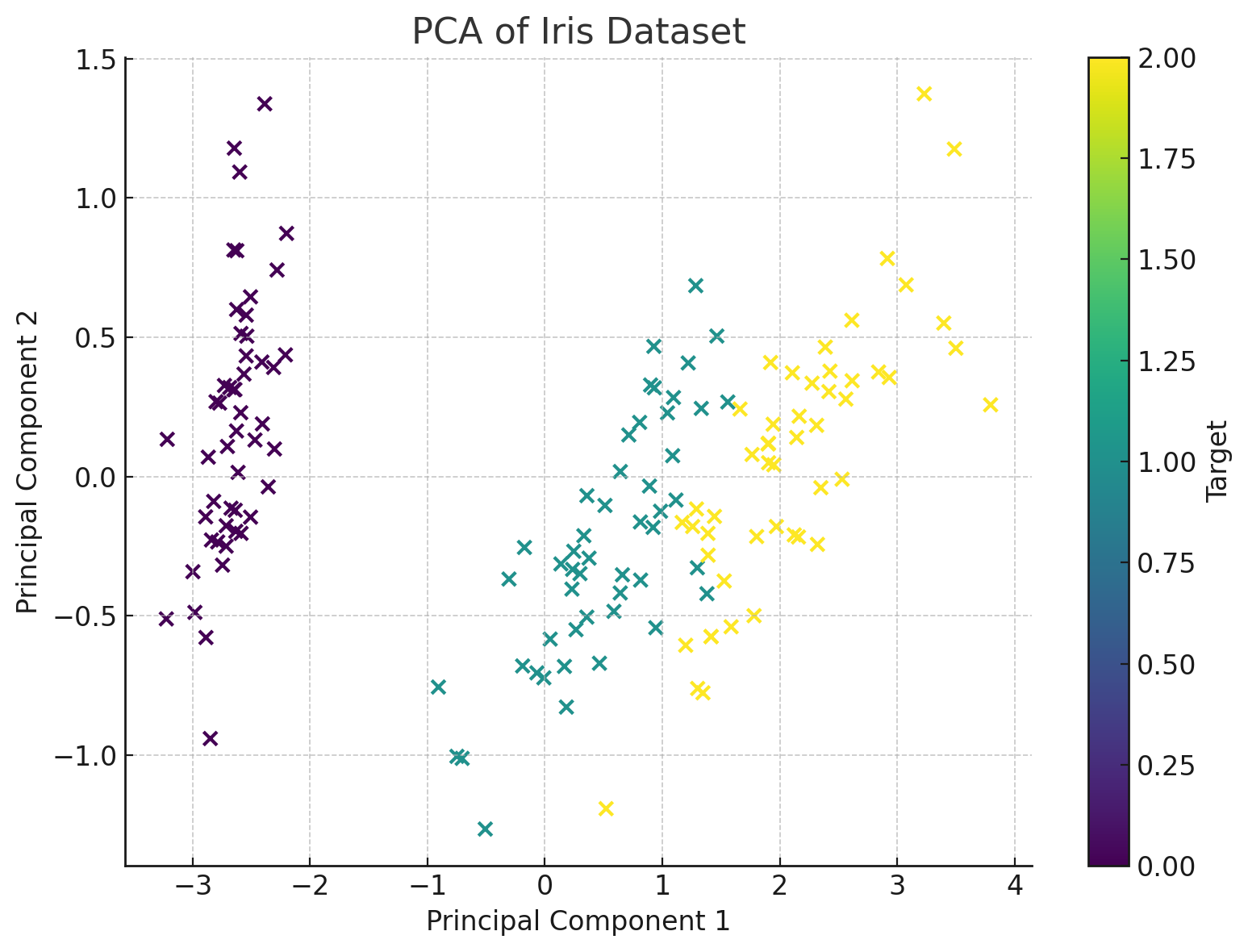
plt.scatter(X_pca[:, 0], X_pca[:, 1], c=y, cmap='viridis')
plt.xlabel('Principal Component 1')
plt.ylabel('Principal Component 2')
plt.title('PCA of Iris Dataset')
plt.show()

Mathematical basis of PCA

Standardize the Data

1. Subtract the mean from each feature to center the data around zero.
2. Optionally scale the features to have unit variance.

Compute the Covariance Matrix

This matrix captures how features vary together:

where $X$ is the standardized data matrix.

Calculate the Eigenvectors and Eigenvalues

Compute the eigenvectors and corresponding eigenvalues of the covariance matrix. Eigenvectors define the direction of the new feature space (principal components. Eigenvalues indicate the amount of variance explained by each component (and therefore the importance of that component).

Sort Eigenvectors by Eigenvalues

Rank eigenvectors (principal components) by their eigenvalues (explained variance). Select the top $k$ to reduce dimensionality.

Project Data onto New Feature Space

Transform the original dataset using the selected top $k$ eigenvectors:

Where:

• $X$ is the mean-centered data matrix.
• $W$ is the matrix of top $k$ eigenvectors (principal components).
• $X_{PCA}$ is the transformed lower-dimensional data.

Alternative code example

Here is an example without using the sklearn library:

import numpy as np
import matplotlib.pyplot as plt
from sklearn.datasets import load_iris

# Load the iris dataset
data = load_iris()
X = data.data
y = data.target

# Step 1: Standardize the data (mean-center)
X_meaned = X - np.mean(X, axis=0)

# Step 2: Compute the covariance matrix
cov_matrix = np.cov(X_meaned, rowvar=False)

# Step 3: Compute eigenvectors and eigenvalues
eigenvalues, eigenvectors = np.linalg.eigh(cov_matrix)

# Step 4: Sort eigenvectors by descending eigenvalues
sorted_idx = np.argsort(eigenvalues)[::-1]
eigenvalues = eigenvalues[sorted_idx]
eigenvectors = eigenvectors[:, sorted_idx]

# Step 5: Select top 2 eigenvectors
k = 2
eigenvectors_subset = eigenvectors[:, :k]

# Step 6: Project data onto the top 2 eigenvectors
X_reduced = np.dot(X_meaned, eigenvectors_subset)

# Plot the manually computed PCA
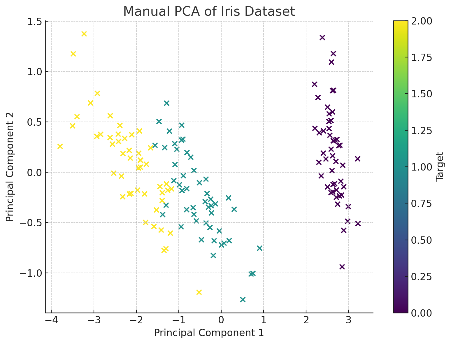
plt.figure(figsize=(8, 6))
scatter = plt.scatter(X_reduced[:, 0], X_reduced[:, 1], c=y, cmap='viridis')
plt.xlabel('Principal Component 1')
plt.ylabel('Principal Component 2')
plt.title('Manual PCA of Iris Dataset')
plt.colorbar(scatter, label='Target')
plt.grid(True)
plt.tight_layout()
plt.show()

See also

internal and external references